
EnergyHub Team
April 24, 2018
In a previous post, EnergyHub’s VP of Analytics Ben Hertz-Shargel dispelled a few exaggerated claims that are frequently made about artificial intelligence (AI) products in the demand response and energy efficiency spaces. We demonstrated that physics implies hard limits on how much load shed or energy savings can be achieved while keeping temperatures within customers’ comfort bands.
So what can AI deliver in these domains? While it can’t miraculously eliminate load, AI does enable fine-grained control of load shape that can be highly beneficial to utilities. As utilities increasingly face complex, time-dependent costs and risks, there is major value in achieving the right load shape for the use case at hand.
The economic and grid stability value of firm reduction
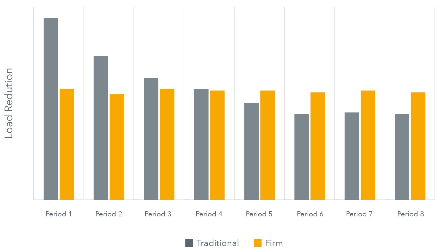
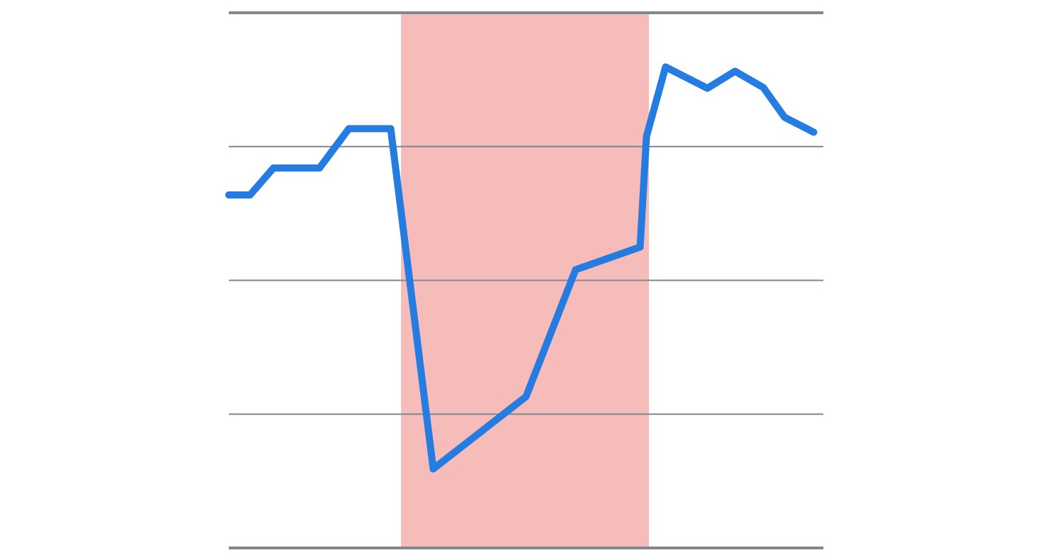
With demand response, there are a number of contexts where steady load shed (which we’ll call “firm reduction”) is desirable. Broadly, firmness matters when we don’t know in advance which time interval during the event will be most critical for reduction. The plot below separates a demand response event into eight time periods of equal length and contrasts firm reduction with the type of uneven reduction that’s common in demand response events (more on this later). The non-firm reduction provides greater reduction during the first half of the event, but leaves the utility seriously exposed if a later period of the event turns out to be the most critical one.
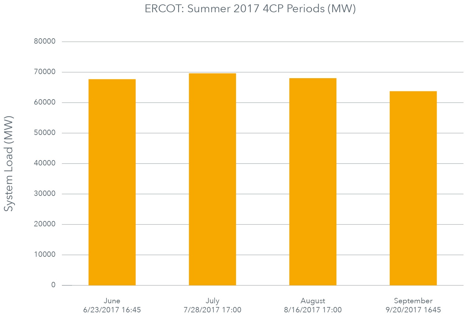
This issue crops up across multiple utility operational areas, and in relation to different forms of risk. For example, a utility may be subject to a transmission charge based on load during peak demand periods. These might be the coincident peaks (CP) of the transmission system or the utility’s own non-coincident peak wholesale demand. The plot below illustrates ERCOT’s 4CP periods for summer 2017, as an example of the former; these four system-wide peak periods were used to assess transmission charges for distribution service providers last year.
Whether the transmission charge is based on coincident or non-coincident peak, the point is that reduction is most critical during the peak interval(s), which solely determine the cost to the provider. The timing of the peak isn’t known in advance, so if demand response can deliver firm reduction across a wider event window that’s expected to contain the peak period, it will mitigate the cost risk.
Distribution peak management is another context where unpredictable peaks pose risks for utilities. Severe peaks can impact the stability of the distribution infrastructure, and regardless of the sophistication of a utility’s planning and operations forecasts, uncertainty in peak timing will always remain. Demand response that achieves firm reduction can serve as an insurance policy against the impact of these peaks, ensuring that demand response capacity is evenly distributed over high-risk periods.
Finally, delivering firm reduction offers economic benefits when utilities are subject to capacity obligations, such as resource adequacy or when they have bid their demand response resource as a market product. In those cases, there are often strict performance penalties for insufficient load shed during any period of an event called by the ISO/RTO. Firm reduction lessens the exposure to these penalties, particularly when there is no reward for over-performance in a given interval.
Dimensions of demand response performance
To understand how AI can deliver firm reduction, let’s be a bit more quantitative about what firm reduction is.
Rather than working with load curves themselves, we’ll work with the reduction curve, which is the population baseline minus the load curve. The reduction curve naturally decomposes as a sum of three components:
- A flat line (the “zeroth-order” component of the reduction curve)
- A line with some slope, but with mean zero (the first-order component)
- A curve with mean zero and no average slope, containing the remaining curve variation (the second-order component)
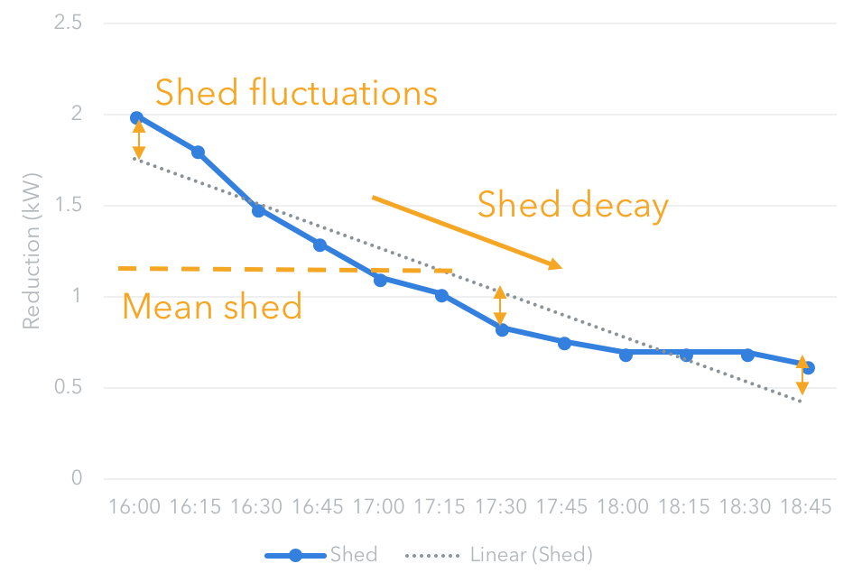
Mathematically, these components represent independent dimensions in the space of timeseries, capturing distinct aspects of reduction curves. As reflected in the following diagram, they naturally give rise to three metrics for demand response performance:
- The mean of the zeroth-order component indicates mean shed
- The size of the slope of the first-order component measures shed decay
The average size of the second-order component is a further metric of shed instability that captures short term shed fluctuations.
With that in mind, we may define firm reduction as load shed that minimizes both shed decay and shed fluctuations. Of course, we’d like to achieve this while also maximizing mean load shed, so we ultimately care about all three performance metrics.
Traditional demand response performance
Now that we have a clearer sense of the metrics of demand response performance, we can explore whether there’s room for improvement on traditional demand response methods.
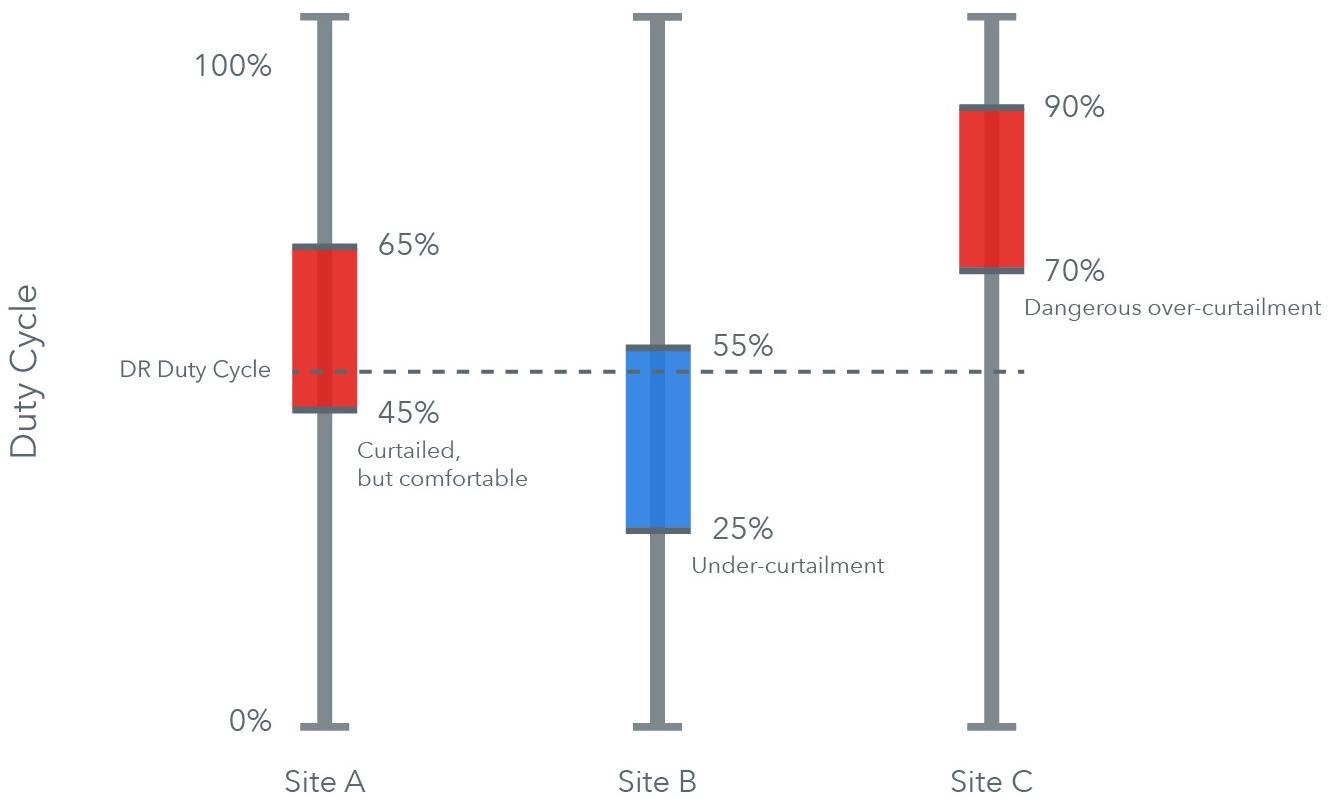
Cycling demand response events employ direct control over the air conditioner’s compressor to maintain fleet load at a constant level. This is not the same thing as achieving constant load shed, however, since the baseline is virtually never constant. Cycling events also can’t offer any guarantees about their effect on the temperature of customers’ homes. This allows potentially drastic impact on customer comfort, and also causes basic inefficiencies. To see why this is the case, keep in mind that the in-home temperature that results from cycling at, say, 50 percent depends on the thermal properties of the home. One customer’s home may require a duty cycle of around 80 percent to maintain an acceptable indoor temperature during the event and will be dangerously over-curtailed by a 50 percent cycling event. Another customer might be comfortable at a 25 percent duty cycle, due to good insulation or a powerful air conditioning unit; a 50 percent cycling event would leave load shed on the table by under-curtailing this customer. The wide variation in thermal properties of homes ensures that almost all customers will be either under-curtailed or over-curtailed to some unpredictable degree. The one-size-fits-all approach of cycling events is neither efficient nor safe.
A demand response strategy that uses temperature setbacks, on the other hand, guarantees customer comfort while allowing a utility to meet its load shed target. However, that strategy tends to exhibit pronounced load shed decay. Traditional setback demand response dispatches all thermostats at the beginning of the event, meaning most homes’ temperature will be well below the increased thermostat setpoint when the event begins. This results in a sharp reduction in load. As the event progresses, thermostats begin to reach their demand response setpoint and cycle on, rapidly diminishing the population reduction. The following load curve is representative of this dynamic:
AI is a versatile tool in demand response
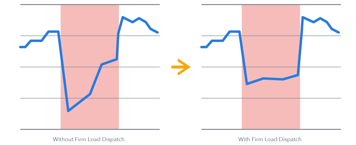
If we want to avoid load shed decay, one of the first ideas we might consider is to stagger device dispatch dispatch; in this approach, some devices are dispatched at the beginning of the event, and as those devices cycle on later in the event, additional devices are dispatched to prevent shed decay. This sounds like a reasonable plan, but introduces an important problem: Every device responds differently to dispatch, and the number of possible dispatch schedules depends exponentially on the number of devices — how do we find the best one?
EnergyHub’s Firm Load Dispatch feature leverages AI to solve this problem. Remember that we ultimately care about achieving firm reduction, as defined in terms mean reduction, shed decay, and shed fluctuations. We combine these into a firmness metric that rewards mean reduction and penalizes shed decay and fluctuations. To evaluate a dispatch schedule in terms of this metric, then, we need a way of determining the load curve it would give rise to. Firm Load Dispatch achieves this by learning thermal models for each home and its air conditioning unit(s), enabling simulation of each site’s load under dispatch. It then uses stochastic optimization techniques to explore the space of dispatch schedules, selecting the one that optimizes the firmness metric.
The best laid plans of model-based optimization can sometimes go awry, so Firm Load Dispatch takes measures to directly mitigate model risk. Thermal models and weather forecasts are never going to be perfect, and it would be problematic if Firm Load Dispatch made that assumption. Instead, the algorithm directly incorporates model and weather forecast noise via Monte Carlo simulation, evaluating dispatch schedules under a range of possible outcomes. This ensures the selected schedule is not only optimal according to our firmness metric, but robust to real-world conditions.
Dispatch schedule tradeoffs
The plot below summarizes the dispatch schedule for an actual Firm Load Dispatch event. Each tick on the y-axis represents a single device; along the corresponding horizontal line, green represents pre-dispatch time and blue represents post-dispatch time (so for a traditional demand response event, the whole plot would be blue). The proportion of green area represents the proportion of control time saved by Firm Load Dispatch across the fleet, relative to a traditional demand response event. In this case, Firm Load Dispatch curtailed for 25 percent less time than a traditional event.
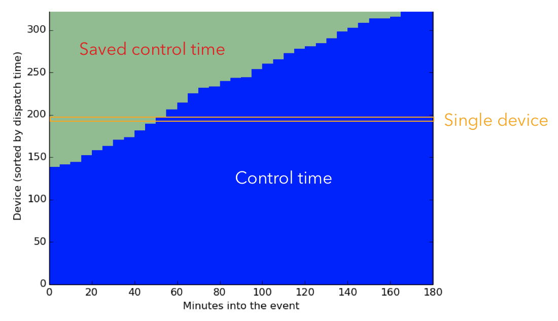
Of course, less curtailment means less total load shed. The existence of saved control time means that an Firm Load Dispatch event will have lower total load shed than a traditional setback demand response event with the same setback. As we’ve discussed, there is no way for AI to increase load shed—only shape it. In fact, we only pay a small price in mean load shed to achieve firm load shape and improve customer comfort. Firm Load Dispatch typically achieves 85 to 90 percent of the load shed of a comparable traditional demand response event while reducing overall device control time across the target population by an average of 20 percent.
The obvious upside of saved control time is improved customer comfort; on average, customers experience a shorter demand response event. Indeed, empirically this has also led to consistently lower opt out rates in Firm Load Dispatch events: Multiple randomized controlled trials (RCTs) have demonstrated, on average, a 25 percent reduction in opt outs with Firm Load Dispatch.
AI can shape load, it cannot eliminate it
AI has a lot to offer in the world of demand response. It’s important to remember, though, that the core value proposition of these techniques is not to increase total load shed. As shown above, basic physics dictates that there’s only so much load shed that can be obtained within the constraints of customer comfort. However, AI enables fine-grained control of load shape, which makes it possible to extract the most value from demand response.
Read “Where AI pushes up against fundamental physics in demand response,” by EnergyHub VP of Analytics Ben Hertz-Shargel.


Interested in keeping up with the latest dispatch from the grid edge?
Get our next post in your inbox.