Where AI pushes up against fundamental physics in demand response

Over the last several years, “artificial intelligence” and “machine learning” have joined “IoT” and “DER” as buzzwords in the utility lexicon. Typically introduced by software vendors, these areas of advanced analytics are breathlessly proclaimed to be revolutionizing numerous areas of the utility business, from power flow optimization to customer bill analytics. Demand response and energy efficiency is no exception, with vendors in this space often making aggressive product claims in presentations and white papers, backed up by little more than their claimed advanced analytics capabilities. Utility program managers and procurement specialists are left to sift through claims and buzzwords, attempting to sort fact from fiction.

EnergyHub’s software leverages advanced analytics, so we have a vested interest in helping utilities get up the AI learning curve. Smarter utility procurement means a more efficient and level playing field, which ultimately benefits both utilities and vendors. To that end, let’s explore a couple typical product claims demand response and energy efficiency vendors make, what the reality is, and how AI can bump up against fundamental physics in delivering results. We’ll also walk through how to spot cherry-picked data in demand response performance results and tough questions program managers and procurements teams should put to vendors about their results.

Let’s begin with a typical demand response claim:

Claim 1: Artificial intelligence unlocks up to 90% load shed during thermostat demand response events

The simple reality is that load shed of this magnitude is not possible under real demand response conditions without severely impacting the customer. This fact comes from basic physical principles and cannot be overcome with analytics. Vendors who make claims like this rely on cherry-picked data, either in terms of the conditions under which demand response happens or the event parameters themselves.

To understand why load shed in the neighborhood of 70-90% isn’t possible, consider that under real demand response conditions — late afternoon or evening on a hot summer day — there is a large temperature gap between the outdoor temperature and the top of the customer’s comfort band, defined as the range of indoor temperatures deemed acceptable to the customer. Demand reduction is achieved by raising the indoor temperature from the bottom end of this band — where the customer has likely set it — to the top. This yields a temporary off cycle for the compressor, as the temperature rises, and then a reduced duty cycle at the new, higher indoor temperature. The demand response control technology determines whether this temperature change is achieved through manipulation of the thermostat setpoint or the compressor cycles themselves, and AI optimization can play a role in coordinating those actions throughout the event and across the aggregation.

Regardless of the dispatch mechanism and timing, however, what remains critical is the outdoor temperature gap. It imposes a minimum duty cycle on the compressor that is necessary to keep each home in the customer’s comfort band over timescales of an hour or more. Under demand response conditions, this duty cycle is typically at least 50 percent. An average load shed in the vicinity of 90 percent with respect to baseline consumption would require duty cycles far below this minimum for most homes, causing indoor temperatures to soar beyond the customers’ comfort bands. This limitation holds regardless of the demand response control technology and AI used to optimize dispatch.

Put simply: AI can shape load, but it cannot eliminate it.

Armed with these basic facts, let’s examine the type of results demand response providers typically put forward to support this type of claim. Figure 1 below shows load and temperature time series data surrounding a demand response event, along with a claim of 2 kW per device load shed achieved.

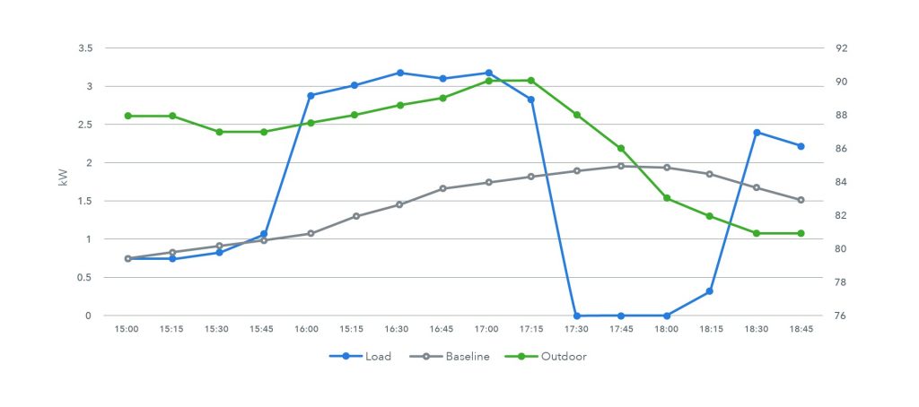
Figure 1: Example demand response vendor data

Four key observations can be made. First, the 2 kW number represents the maximum load shed, not the average or other representative central statistic. Second, this was only a 1-hour event, and average load shed generally decays with event duration, so the results cannot be extrapolated to longer events. Third, observe that the event plays out over unrealistically mild outdoor temperatures. EnergyHub clients typically call demand response events at temperatures above 90 degrees, when HVAC meaningfully contributes to system load. Moreover, the outdoor temperature is actually plummeting during the event, reaching the low 80s by the 45-minute mark, easing the cooling burden precisely when load would otherwise be expected to pick up. Finally, an hour-and-a-half precool is evident in the data, which is longer than typical demand response precools, particularly given the short event duration. Utilities often cannot afford such a long precool, either due to short-term dispatch notification or the impact on customer bills. In any event, as with the 1-hour duration and mild weather, such a long precool precludes extrapolation of results to events with shorter or no precool.

Our observations are summarized in the following list of questions utilities should consider when evaluating demand response results, even those in third-party analyses:

1. What load shed metric is used to report performance?
2. Are the events as long as the ones the utility will call during their program?
3. Are weather conditions reported, and, if so, are they typical of the utility’s demand response events?
4. Is a precool employed, and does it match the duration and temperature offset of the precool expected in the program?

Let us now turn to a second claim, this one around energy efficiency:

Claim 2: Leveraging artificial intelligence and thermal modeling, vendor’s platform can achieve significant energy savings while keeping the home within 0.5-1.0 degree of its usually scheduled temperature.

This type of claim is more complicated to evaluate, taking us deeper into HVAC physics. The key point to note is that, regardless of modeling and optimization strategy, the energy savings produced by an HVAC control strategy that keeps indoor temperature within a small setback cap of the customer’s schedule can be no greater than the savings achieved by simply applying that fixed setback cap to the schedule. There is a broad literature documenting the impact of small, fixed setbacks on energy efficiency, typically showing relative savings of a few percent — hardly significant, and not owing to the analytics.

To understand the italicized point further, consider Figure 2, which illustrates heat flow in a home. Fourier’s law of conduction says that heat flow between two bodies is proportional to their temperature difference, in this case the temperature gap T_out – T_in. In order to maintain the indoor temperature, the air conditioner must evacuate (through its refrigerant) as much heat as leaks in through the home’s envelope. In other words, the temperature gap directly implies the amount of work the air conditioner must do, which grows with the size of the gap.

It turns out that the efficiency of the air conditioner — the factor that determines how much electrical energy is needed to achieve this useful work — is also a function of the indoor and outdoor temperatures, and decreases as the temperature gap increases. Putting these two facts together: The energy consumed by the air conditioner is a function of the indoor and outdoor temperatures, and grows with the temperature gap.

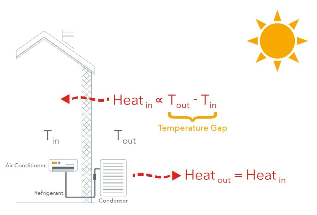
Figure 2: Heat flow through a building envelope and the dependence of HVAC heat evacuation on the outdoor temperature gap

Compare now the optimized control strategy in the claim with the simple strategy that adds the fixed setback cap to the customer’s schedule. The former strategy has a temperature gap greater than or equal to the latter’s at all times, and therefore must consume at least as much energy.

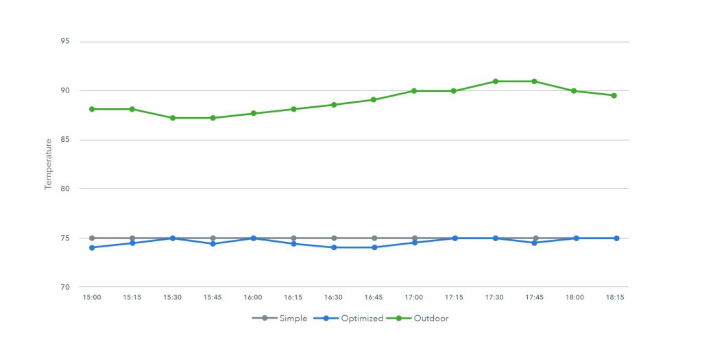
Figure 3: The temperature gap under the optimized strategy is always greater, so it must use more energy.

Again, the conclusion is based on physics and holds regardless of modeling and optimization. The conclusion also holds when one accounts for other sources of heat gain in the home, such as insolation, lighting and appliance use. The excess heat simply increases the amount of heat the air conditioner must evacuate under both strategies, and is equivalent to raising the outdoor temperature.

As the analysis of these two typical claims has showed, AI and other advanced analytics techniques cannot overcome fundamental physics. Utilities and other grid operators should therefore bring a critical eye to aggressive product claims that hinge on them, ask tough questions and consider the underlying physics involved. 

All this is not to say that AI does not offer tremendous value to demand response and other grid services, of course. In an upcoming blog post we will address precisely why it does, and explore the multiple dimensions and critical tradeoffs of demand response performance.